One of Picterra’s main focuses is to provide not only easily accessible but also easily understandable machine learning tools to our users. To that end we’re experimenting with methods to understand how the detector is “thinking” in order to help our users make more powerful detectors.

Until now the only method to interact with a model was to run it on images, observe the predictions, and then try to reason why the model was making certain mistakes. This is analogous to attempting to understand what a student has learned based on only their answers from an exam. But imagine that instead of just having the final answer, we can also look into their brain to better understand how confused or confident the student is in their responses. This would allow us to have better strategies in order to more effectively guide the student.

Likewise for your detector we are working towards allowing your model to understand which regions of your imagery it is more confused about by providing a “confidence map”. This map,  in combination with detection results on that same imagery, can be used to better inform your next decision on how to add more training areas to your dataset. To generate the confidence map, we use a technique inspired by [1] because it offers a simple framework to obtain a confidence map without significantly changing the underlying structure of our model. The idea is quite simple: run the model multiple times but keep the dropout layers during prediction. This means that each time the model is run we will have a distinct prediction map and thus we can compute the uncertainty/confidence level of the different iterations. We experimented with two methods of aggregating the multiple run: the first was to take the variance for each pixel and the second was based on entropy[2].

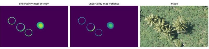
Example of confidence maps on a coconut tree detector (yellow means less certain)

We can see with this example that:

• The two maps look similar (they are based on the same set of runs just with the two different aggregations approaches).
• The model seems to be uncertain on the edge of each prediction which is expected since even for humans it is the hardest part to annotate.
• We also see that the model seems to be less certain about one coconut tree in particular.

Discovering missing annotations

To have a better understanding of what is going on we will add the prediction of the model.

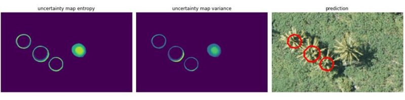
We see that the “uncertain coconut tree” is not detected by the model. In this specific case the issue was that the model used this image (and others) to train but the “missing” coconut tree was not annotated and using the confidence map helped us notice the issue on this dataset.

We decided to explore this concept of discovering missing annotations more closely by using another dataset where roughly half of the annotations were removed to see if we can replicate this behavior.

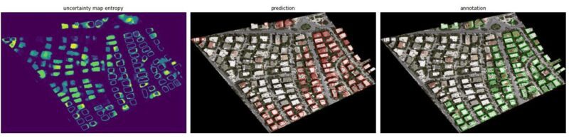
We observe here that the model is not detecting non annotated buildings since it is still highly uncertain on the majority of them. Therefore we can conclude that discovering missing annotations in your training areas could be a first use case for confidence maps; trying to curate an annotated dataset.

Dataset recommendations

One other (and potentially more appealing use case) is to help our users build better detectors by using confidence maps to choose new spots to annotate. Indeed we can use confidence maps in several ways:

• Try to find false negatives (i.e., missing detection) by observing the confidence map and looking for “blobs” of uncertainty.
• If we observe a missing prediction with no uncertainty attached to it, this could mean that it’s a hard false negative.
• We may want to look more closely at prediction where the model is uncertain about the full object and not just the edge. It could indicate a false positive (i.e., wrong prediction).
• … and many more to discover!

To validate our hypothesis we conducted an experiment.

We chose one dataset (seals dataset) and removed half of the 40 training areas (baseline). The goal is to choose just a few new training areas (here adding only 5 new ones) using confidence maps to get the best score possible.

First, we will obtain the score (for our case foreground iou and f-score) for the half and full dataset. We then compared two approaches:

• Just looking at the model prediction on potential new training areas.
• Using prediction and confidence map on potential new training areas.

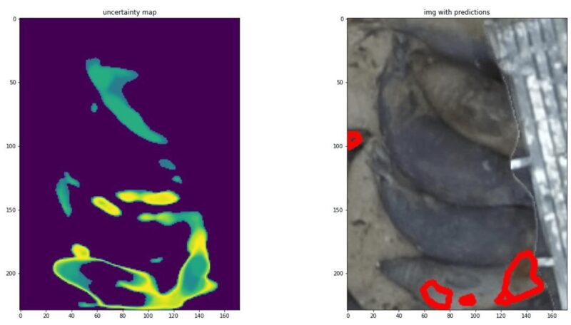
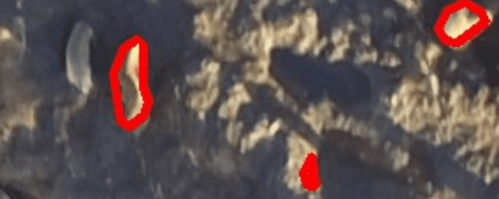
Example of input (in this case just looking at predictions guide us to choose this area).

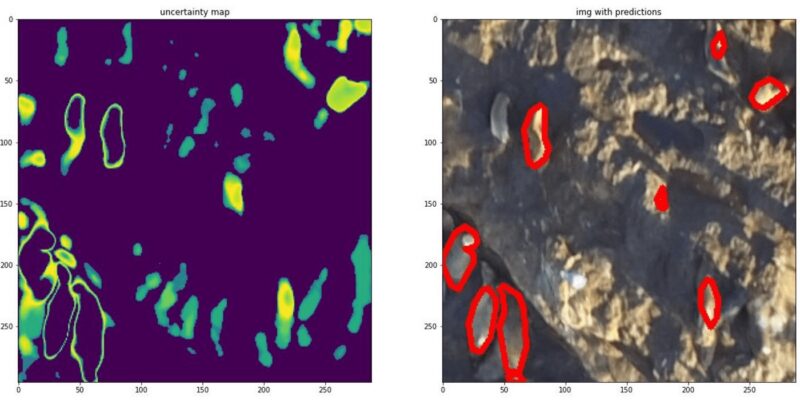
Example of input (confidence map gives us insight on what can be confusing for the model) even though the detections look better here, the model is still quite unsure in a lot of areas, so it may still be wise to add a training area here.

Given the same dataset a trained model can vary due to the nature of how the data is randomly sampled from within your dataset. To get a more representative score it is better to train multiple models to see if one setup is consistently better than another. We decided to train the same model multiple times on each dataset and compare each experimentation using a standard boxplot. From left to right in the image below we have 4 experiments.

• Baseline – The control test using a fixed dataset.
• Without confidence map – Adding 5 more training areas from a fixed set of possible new training areas to add to the baseline using only the models output as a guide on how to choose from said set.
• With confidence map – Adding 5 more training areas from the same fixed set, but this time using confidence maps on those areas as additional information.
• Full dataset – Using the entire set of possible new training areas for comparison.

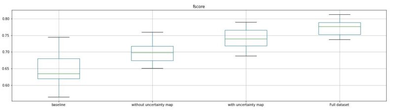
The horizontal axis represents the experimentation, vertical axis the fscore.

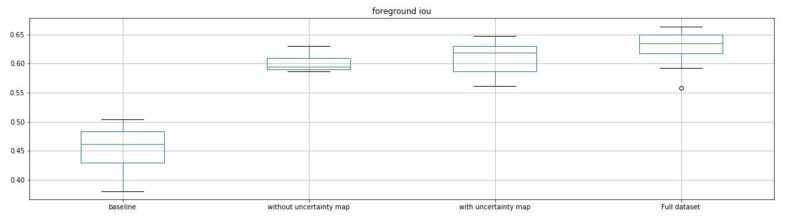
The horizontal axis represents the experimentation, vertical axis the foreground iou score.

We can see that just adding 5 training areas increases drastically the overall score and that using the confidence map with the model prediction performs better than just using the raw prediction.

This is a good first indication that the confidence map can be used to make better informed decisions on what should be added to your dataset, or in other words, to provide a dataset recommendation!

Conclusion

In this article we have presented an approach to make more informed decisions on which part of an image it would be the most useful to annotate in order to improve a detector. This feature is definitely still in an early RnD phase. There’s plenty more experimentation to perform on our end to make sure that the methodology is sound and stable. Likewise, there’s plenty of brainstorming to perform on how we can best let our users benefit from our work here at Picterra. However, between experimentation and brainstorming we hope to provide our users with a functioning version of this feature within the coming months.

This is an exciting new addition to Picterra’s machine learning toolbox and we can’t wait to see what it evolves into, so stay tuned for more details!

[1] Gal, Y., & Ghahramani, Z. (2016, June). Dropout as a bayesian approximation: Representing model uncertainty in deep learning. In international conference on machine learning (pp. 1050–1059). PMLR.

[2] Clément Dechesne, Pierre Lassalle, Sébastien Lefèvre. Bayesian Deep Learning with Monte Carlo. Dropout for Qualification of Semantic Segmentation. IGARSS 2021 — IEEE International Geoscience and Remote Sensing Symposium, Jul 2021, Brussels, Belgium. hal-03379980