Importing Zurich’s WMS
The first thing we need to do is import our data source. In this case, data comes from a Web Map Service (WMS), namely Zurich’s open WMS. The city kindly provides open and free access to use aerial photography of Zurich in 2018, and that’s what we’ll use for this project.
We have also created a web page that lists known open WMS and lets you import them directly into Picterra: https://old.picterra.ch/imagery/. We’ll simply open this page, click on Zurich’s thumbnail, and hit the “Import into Picterra” button.

If you have an open WMS that you’d like to use, just let us know and we’ll happily add it to this list.

Then, let’s zoom over a large region of interest and import that as our image. The resulting raster is 18996MP and covers an area of 189.91 km².

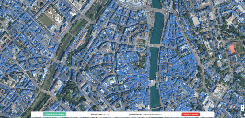
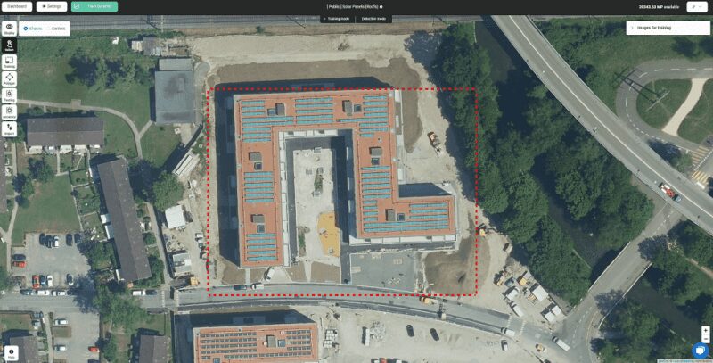
If we just run this detector over the whole image, it would process areas that are known to be free of solar panels (such as lakes, forests, roads). In cases like this, where you know where to look (in our case, rooftops), you can import detection areas to tell the detector to process only given areas. Thankfully, we have access to Zurich’s building footprints, so let’s import them. Open the “Info” popup on the raster, hit “manage detection areas” and upload a geojson file containing all buildings’ footprints. You’re ready to start solar panel monitoring.
This results in a raster that is now only 2796MP, an 86% reduction in processing size and time.

The next step is to create our detector. We have already covered in other blog posts how to create efficient detectors, so here are a couple of annotations and training/testing areas we’ve defined.
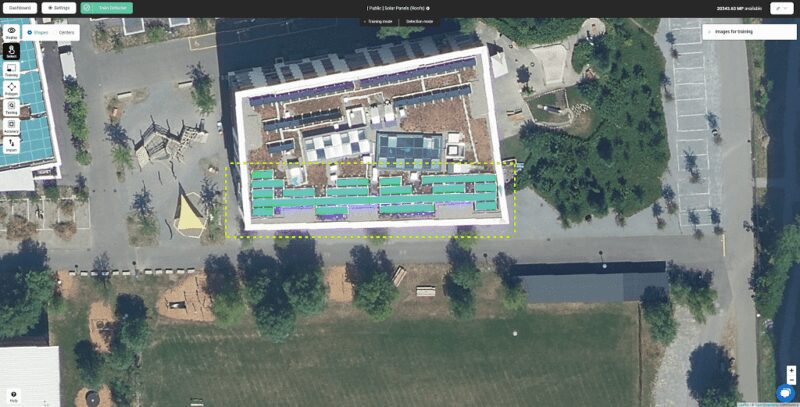
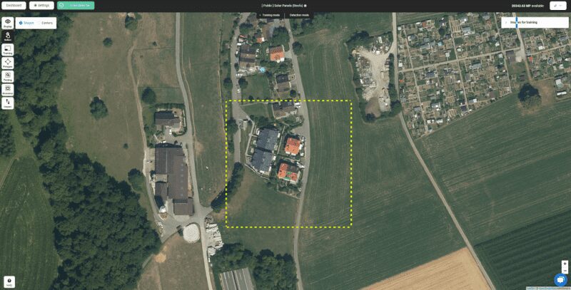

Then comes a train/improve iterative loop, where we’ll refine our detector by improving the annotations and training areas we feed it until we are satisfied with the results seen in our testing areas.
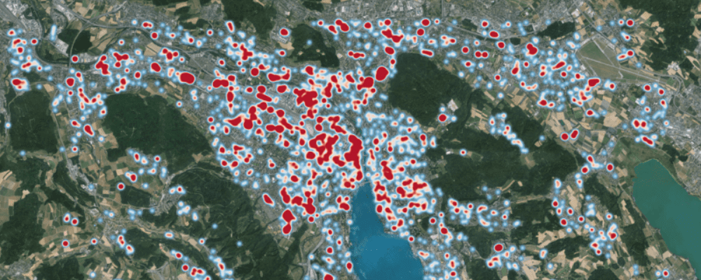
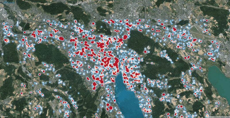
Once done, let’s run our detector on the whole raster and export the results as a Mapbox heatmap for a nice visualization of solar panel monitoring.
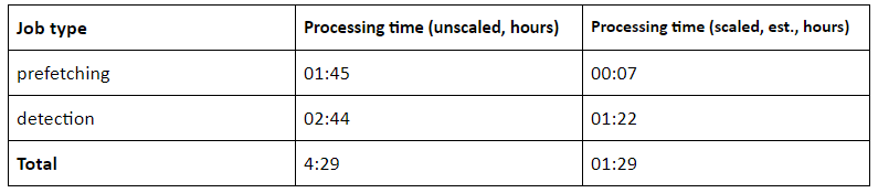
Here is a little breakdown of how much time was spent during this detection:
We also ran this detector without detection areas for comparison:
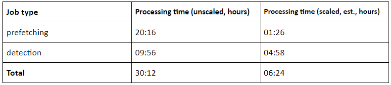
“Prefetching” happens when our system downloads all the WMS data needed for detection. Because we cache it, it can get reused across runs, so comparing both prefetching times does not make a lot of sense. It is still interesting as an indicative number.
Note the difference between unscaled durations and estimated scaled durations. When large jobs land in our processing queue, our infrastructure scales its number of workers to work in parallel, reducing the processing time. The “unscaled” column lets you see how long each run would have taken, had we not scaled the infrastructure. The “scaled” column lets you see how long it takes when the infrastructure scales at its maximum capacity. To give you an idea, we currently use 14 workers for prefetching, and 2 for detection.